OSPF (Open Short Path First) Routing Protocol implemented using Dijkstra Algorithm

What is Routing Protocol?

Let us try to understand this concept

Suppose you want to go to your shop from home. You book a cab or take an auto to your shop. In the path of your journey, your auto driver encounters several signboards which help him/her to take the proper turn or best path, or in the case of a cab, Google Maps will help you in choosing the best route. In this likeness consider yourself as the Data the auto or cab as the Routed Protocol, and the signboards or the GPS installed in your driver’s phone as the Routing Protocol.

Similarly, It provides appropriate addressing information in its internet layer or network layer to allow a packet to be forwarded from one network to another.

The IP network is classified into two categories: Interior Gateway and Exterior Gateway Protocol

Interior gateway protocols are used inside an organization’s network and are limited to the border router. Exterior gateway protocols are used to connect the different Autonomous Systems (ASs). A simple definition that fits most of the time defines the border router as a router that has a foot in two worlds: one going to the Internet and another that is placed inside the organization and that’s why its name is, border router.

Purpose and Use Cases

With Dijkstra’s Algorithm, you can find the shortest path between nodes in a graph. Particularly, you can find the shortest path from a node (called the “source node”) to all other nodes in the graph, producing a shortest-path tree.

This algorithm is used in GPS devices to find the shortest path between the current location and the destination. It has broad applications in industry, especially in domains that require modeling networks.

What is OSPF(Open Shortest Path First)?

OSPF is a link-state protocol that uses a shorted path first algorithm to build and calculate the shortest path to all known destinations. The shortest path is calculated with the use of the Dijkstra algorithm. The algorithm by itself is quite complicated. This is a very high-level, simplified way of looking at the various steps of the algorithm.OSPF is not a CISCO proprietary protocol like EIGRP.OSPF always determines the loop-free routes. If any changes occur in the network it updates fast.

These are some of the important points related to OSPF.

1. The OSPF is an open standard protocol that is most popularly used in modern networks.
2. It is used to find the best path between the source and the destination router using its own Shortest Path First.
3. Various protocols are used for the shortest path. But in real life mostly problems are undirected graph-like nature. OSPF using Dijkstra’s algorithm solved the shortest path problem in both types of problems i.e. directed and undirected graphs.

Shortest Path First Algorithm

OSPF uses a shorted path first algorithm to build and calculate the shortest path to all known destinations. The shortest path is calculated with the use of the Dijkstra algorithm. The algorithm by itself is quite complicated.

Routing protocols like OSPF calculate the shortest route to a destination through the network based on an algorithm.

Why there is a need for OSPF when there is RIP protocol?

The first routing protocol that was widely implemented, the Routing Information Protocol (RIP), calculated the shortest route based on hops, that is the number of routers that an IP Packet had to traverse to reach the destination host. RIP successfully implemented dynamic routing, where routing tables change if the network topology changes. But RIP did not adapt its routing according to changing network conditions, such as data transfer rate. Demand grew for a dynamic routing protocol that could calculate the fastest route to a destination. OSPF was developed so that the shortest path through a network was calculated based on the cost of the route,

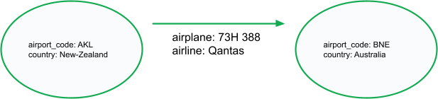
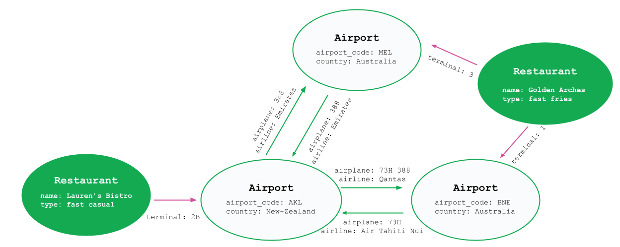
OSPF is a routing protocol. Two routers speaking OSPF to each other exchange information about the routes they know about and the cost for them to get there.

When many OSPF routers are part of the same network, information about all of the routes in a network is learned by all of the OSPF routers within that network—technically called an area.

Each OSPF router passes along information about the routes and costs they’ve heard about to all of their adjacent OSPF routers, called neighbors.

OSPF routers rely on the cost to compute the shortest path through the network between themselves and a remote router or network destination. The shortest path computation is done using Dijkstra’s Algorithm This algorithm isn’t unique to OSPF. Rather, it’s a mathematical algorithm that happens to have an obvious application to networking.

The routers work on the third layer of our OSI model. OSPF is a routing protocol. When data move across multiple networks, IP routing helps to determine the path of data by setting some protocols to reach the source destination. RIP (Routing Information Protocol) and OSPF (Open Shortest Path First) Protocol are types of dynamic routing.

Comparing the difference between Static and Dynamic Routing :

– Static routing is for small networks like small scale organization that has predicted number of users and static or minimum bandwidth usage

– Dynamic Routing is used in the case of large networks because of its capabilities like it keeps changing and updating along with network topologies. Dynamic Routing Protocols dynamically discover network destinations.

OSPF maintains information in three tables:-

Topology Table contains the entire road map of the network with all available OSPF routers and calculated best and alternative paths. 

Neighbor Table that contains information about neighboring routers so that information can be interchanged.

 Routing Table where the current working best paths will store and it is used to forward the data traffic between neighbors.

How Dijkstra’s Algorithm Works With Example

Consider the map below. The cities have been selected and marked from alphabets A to F and every edge has a cost associated with it.
We need to travel from Bengaluru to all other places and we have to identify what are the shortest paths with minimal cost from Bengaluru to other destinations.

Working of Dijkstra’s Algorithm

• Convert the problem to its graph equivalent.

Upon conversion, we get the below representation. Note that the graph is weighted and undirected. All the cities have been replaced by the alphabets associated with them and the edges have the cost value (to go from one node to another) displayed on them.

Example Problem of Dijkstra’s Algorithm Working Part 1

• Assign a cost to vertices.

Assign a cost of 0 to source vertex and ∞∞ (Infinity) to all other vertices as shown in the image below.
Maintain a list of unvisited vertices. Add all the vertices to the unvisted list.

Example Problem of Dijkstra’s Algorithm Working Part 2

• Calculate the minimum cost for neighbors of the selected source.

For each neighbor A, C, and D of source vertex selected (B), calculate the cost associated to reach them from B using the formula. Once this is done, mark the source vertex as visited (The vertex has been changed to blue to indicate visited).

Minimum(current cost of neighbor vertex, cost(B)+edge_value(neighbor,B))

1. For neighbor A: cost = Minimum(∞∞ , 0+3) = 3
2. For neighbor C: cost = Minimum(∞∞ , 0+1) = 1
3. For neighbor D: cost = Minimum(∞∞ , 0+6) = 6

Example Problem of Dijkstra’s Algorithm Working Part 3

• Select the next vertex with the smallest cost from the unvisited list.

Choose the unvisited vertex with minimum cost (here, it would be C) and consider all its unvisited neighbors (A, E, and D), and calculate the minimum cost for them.

Once this is done, mark C as visited.

Minimum(current cost of neighbor vertex, cost(C)+edge_value(neighbor,C))

1. For neighbor A: cost = Minimum(3 , 1+2) = 3
2. For neighbor E: cost = Minimum(∞∞, 1+4) = 5
3. For neighbor D: cost = Minimum(6 , 1+4) = 5

Observe that the cost value of node D is updated by the new minimum cost calculated.

Example Problem of Dijkstra’s Algorithm Working Part 4

• Repeat step 4 for all the remaining unvisited nodes.

Repeat step 4 until there are no unvisited nodes left. At the end of the execution, we will know the shortest paths from the source vertex B to all the other vertices. The final state of the graph would be like below.

Where OSPF is Used?

Where OSPF is Used

OSPF is an Interior Gateway Protocol (IGP). As the name suggests, these are used for internal network routing. This would typically be between switches and routers in the same location. Sometimes OSPF has also been used in Layer 2 connections between offices.

OSPF is the most widely used but it is not the only choice. With that said, it is the most standardized IGP and that allows for optimal vendor interoperability. OSPF is primarily used for internal routing because it’s a link-state routing protocol.

OSPF is a Link State protocol based on cost under a single routing solution that maintains information of all nodes on the network. Since each node holds the entire network structure information, each node can independently calculate the path to reach the destination by adopting the shortest path algorithm namely Dijkstra’s algorithm as discussed earlier.

The overhead of being a link-state protocol is minimized due to the smaller topology. Not to say they cannot get large but compared to the topology of internet routing, they are usually minimal.

The benefit to being a link-state protocol is its ability to highly engineer traffic routing due to its in-depth understanding of the topology. Each router has a full view of how each router is connected. The downside is that many convergence scenarios require a full or partial table recalculation.

Thanks For Reading this article…!!!!

Use Case of MongoDB DataBase

What is a Graph Database?

A graph database is a database that stores data in nodes and edges—nodes for information about an entity and edges for information about the relationship or actions between nodes. This data model allows graph databases to prioritize relationships between the data, which makes searching for connections and patterns in the data easier than it is with traditional databases.

Graph databases use the following key terms:

• Nodes (or vertices). You can think of nodes as the nouns in your databases; they store information about people, places, and things.
• Edges (or relationships). You can think of edges as the verbs in your databases; they store information about the actions that are taken between the nodes.
• Properties. A property is a key-value pair that stores information about a particular node or edge.
• Labels. A label can optionally be used to tag a group of related nodes.

The section below contains an example of how data is modeled in a graph database using nodes, edges, properties, and labels.

How is Data Stored in a Graph Database? An Example

Let’s walk through how data is stored in a graph database. Let’s say you want to store air travel information.

Each airport would be represented by a node, and information about the airports would be stored in the nodes’ properties. For example, you could create a node for Auckland Airport in New Zealand with properties such as airport_code: AKL and country: New-Zealand.

A flight between two airports—that is, the relationship between two nodes—is represented by an edge. The edge’s properties contain information about the flight. In this example, you could create an edge between the nodes for Auckland Airport and Brisbane Airport. The edge could have properties like airplane: 73H 388 and airline: Qantas.

A node represents Auckland Airport, with its properties listed. An edge represents a flight from Auckland Airport to Brisbane Airport, with properties for airplane and airline.

In addition to the nodes for airports, you might create nodes for other related entities such as airport restaurants. You might choose to apply a label like “Airport” to the airport nodes and “Restaurant” to the restaurant nodes. The diagram below shows a graph with several nodes, edges, properties, and labels.

A graph that represents airports, airport restaurants, and flights.

Some use Cases of MongoDB DataBase :

Customer Analytics

Creating consistently good customer experiences has become a key challenge for many organizations. The reality is that our expectations around what a good customer experience is has increased dramatically over the past few years. What used to be cool and different is now the norm.  

Data aggregation is one of the keys to creating amazing customer experiences. Companies are collecting massive amounts of data about their existing and potential customers and aggregating it with publicly available data. This data can tell companies how customers interact with products (digitally and in person), personal preferences, demographics, etc. From all of this disparate data, companies can build customer profiles and nurture paths with the goal of getting the customer to buy more products.  

With all of this data coming from different sources with different schemas, tying it all together at such a massive scale is a huge challenge. The flexibility and scalability of MongoDB provides a solution. MongoDB allows for the aggregation of this data and building analytical tools in order to create amazing customer experiences. MongoDB’s speed allows for dynamic experiences that can evolve based upon the customer behavior in real time.

Product Catalog

Product catalogs are not new to the evolving digital experience. What is new is the volume and richness of the data that feeds the interactions in product catalogs that we use today. MongoDB provides a great tool to store many different types of objects with different sets of attributes. MongoDB’s dynamic schema capability allows for product documents to only contain attributes that are relevant to that product. Gone are the days of needing every product record to contain every possible attribute. MongoDB users can very quickly and easily make changes to their catalogs, providing a better experience for developers and customers.

Real Time Data Integration

Companies have vast amounts of data spread across their organization. Data provides value if it’s aggregated in one “single view”. Previously, energy and resources were spent on data ingestion, transformation, and schema changes in order to obtain a single source of data. MongoDB’s flexibility and query capabilities make it easy to aggregate this data and create the tools that make organizations more efficient. This aggregation can be achieved to provide a “single view” of their data in real time. With the addition of change streams in MongoDB 3.6, developers can now monitor and take action on specific events quickly.

Mobility and Scaling

With most mobile application development, companies are dealing with varying data structures coming from multiple sources and potentially highly dynamic growth. The flexibility and scalability of MongoDB provides a great database solution for dealing with this type of environment. With schemas that can evolve over time, mobile application developers don’t have to spend time adjusting the database. Instead, developers can focus on developing the customer experience.

ObjectRocket for MongoDB

Today, modern businesses are thinking about better ways to store and manage their data, gain better customer insights, adapt to changing user expectations, and beat competitors to market with new applications.

MongoDB is a great tool that many companies find useful, but managing MongoDB doesn’t fit into everyone’s business model. It’s hard to find the right expertise and many companies can’t afford to hire the headcount. ObjectRocket for MongoDB can help. No matter where your app is hosted, we can help you get the most from your data.

Some Real-World Companies That Use MongoDB 

1. eBay

eBay is a multinational company that provides a platform for the customer to customer sales. It is currently running a large number of projects in MongoDB like merchandising categorization, cloud management, metadata storage, search suggestions.

2. MetLife

MetLife is a leading company in employee benefit programs, annuities, and insurance. There are more than 90 million customers in the Middle East, Europe, Aisa, Latin America, Japan, United States. MetLife is using MongoDB for its advanced customer service application called The Wall.

This application provides a combined view of transactions, policy details, and other details of MetLife Customers. It looks like Wall of Facebook, which takes data from 70 legacy systems and merges it into a single record. It stores 24 Terabytes of data and runs across six servers in two data centers. MetLife is working on a series of Big Data projects where MongoDB-based applications are part of it.

3. Shutterfly

Shutterfly is one of the most popular online photo sharing, and it is using MongoDB to manage and store more than 6 billion images, which has a transaction rate of up to 10,000 operations per second. Shutterfly earlier used Oracle but later transitioned to MongoDB.

Shutterfly company realized that moving to a non-relational database will help them to increase their scalability, performance, and productivity of the programmer.

Shutterfly did consider many other alternate database systems like BerkeleyDB, CouchDB, or Cassandra. The company has confirmed that they are pleased with their decision of transitioning from Oracle to MongoDB.

Thanks for Reading this article …!!!!

Web-APP For Kubernetes

Hello Learners,

In this Article we are going to implement Kubernetes on the top Web_Application.

so Let’s start

What is Containerization ?

Containerization is the Upgraded version Of Virtualization which provides virtual OS in the form of Containers. These containers are the light weight OS which can be installed, Configured and Boot within a second. The need of Containerization comes when Virtualization cannot help us, if we want to do same setup in 1000 systems we have to install OS which is time consuming task and requires extra resources . Instead if we use Containers it saves time by quick deployment and saves resources.

We use Container Engine to run these Containers and one of mainly used Container Engine is Docker…

Docker is the great tool but there are many cases in which Docker(Container Tecnology) fails to fulfill our demands :

1. If one of the Container OS fails, Docker don’t come to know about it and it can show downtime in App deployed in that OS. Means it cannot monitor OS, we have to do it manually.
2. It requires time and efforts to deploy same setup again if previous OS setup fails and there are higher chances of Human errors .
3. Management of these containers become a challenge for us because we cannot see to it 24/7.

To solve these Issues we came up with a software soution which will Monitor our Containers 24/7 and has a capacity to Launch new container if previous one fails. That is the reason Kubernetes is called as Container Management Tool .

Why use Kubernetes?

Kubernetes helps you to control the resource allocation and traffic management for cloud applications and microservices. It also helps to simplify various aspects of service-oriented infrastructures. Kubernetes allows you to assure where and when containerized applications run and helps you to find resources and tools you want to work with.

Key Features Of Kubernetes

• Kubernetes helps to manage containerized applications in various types of physical, virtual, and cloud environments.
• Automated Scheduling.
• Self-Healing Capabilities
• Automated rollouts & rollback
• Horizontal Scaling & Load Balancing
• Offers environment consistency for development, testing, and production
• Infrastructure is loosely coupled to each component can act as a separate unit
• Provides a higher density of resource utilization
• Offers enterprise-ready features
• Application-centric management
• Auto-scalable infrastructure
• You can create predictable infrastructure

Here is the architecture of Kubernetes :

Guys, See the Below there is page of Our WebApp .

In the You can see a Dashboard with Buttons named Pod, Deployment, Services, PVC and Replica Set…

These are some of the resources of Kubernetes which we have Automated in such a way that even a person who don’t know command can also handle the GUI very well.

Here as you can see there is some Number mentioned below every resource That is the count of Items of that resource. Eg: There are 3 pods are running.

This is a block of Code which will contact to our CGI server and Get the live Count of the Resources for us and display on the Screen .

If we want to do some more actions then run that commands which you want to print.

Like this we did for each resource and finally created a Dashboard for Kubernetes…

This was a Team Task, I would like to Thank all My Teammates for their Support…

Team Members :

1. Pratik Patil

Download the code from Git-Hub :

https://github.com/mtg-tech/summer_task9

That’s it for the Day and stay tunned for more content…

Thanks For Reading the Article …!!!

RTO Image Detection

This is Summer Internship task given by our mentor Vimal Daga Sir, in this task we are going to learn how image processing work and how we can get numerical data from the image.

Task Decription

📌 In this task :
👉Create a model that will detect a car in a live stream or video and recognize characters on number plate of the car .
👉Secondly , it will use the characters and fetch the owners information using RTO API’s .
👉Create a Web portal where all this information will be displayed (using html,css,and js)
📌 Note : You may create your own detection model .
👉 Make a blog/article/video explaining this task step by step.
❄️ Submit the link of blog/article or video link

Download the Code from Git-Hub :

https://github.com/mtg-tech/task_8_summer

Thanks For Watching……!!!!!

Live Streaming Video Chat App without voice using CV2 module of Python

This is a video streaming app so here I am going to upload a video which gives you better idea how this code works.

Get the Code from my Git-Hub Account :

https://github.com/mtg-tech/Task_3

Thanks For Reading….!!!

K-Mean Cluster and it’s Real Use Cases

What is clustering

Clustering is one of the most common exploratory data analysis techniques used to get an intuition about the structure of the data. It can be defined as the task of identifying subgroups in the data such that data points in the same subgroup (cluster) are very similar while data points in different clusters are very different.

Unlike supervised learning, clustering is considered an unsupervised learning method since we don’t have the ground truth to compare the output of the clustering algorithm to the true labels to evaluate its performance. We only want to try to investigate the structure of the data by grouping the data points into distinct subgroups.

What is K-Mean Cluster

K-means clustering is a simple and powerful unsupervised machine learning algorithm that is used to solve clustering problems. It follows a simple procedure of classifying a given data set into a number of clusters, defined by the letter “k,” which is fixed beforehand.

It is a centroid-based algorithm, where each cluster is associated with a centroid. The main aim of this algorithm is to minimize the sum of distances between the data point and their corresponding clusters.

Where to use k-means clustering?

K-means clustering has uses in search engines, market segmentation, statistics and even astronomy.

It is used for clustering analysis, especially in data mining and statistics. It aims to partition a set of observations into a number of clusters (k), resulting in the partitioning of the data into Voronoi cells.

Working of the K-Means algorithm

Step-1: Select the number K to decide the number of clusters.

Step-2: Select random K points or centroids.

Step-3: Assign each data point to their closest centroid, which will form the predefined K clusters.

Step-4: Calculate the variance and place a new centroid of each cluster.

Step-5: Repeat the third steps, which means reassign each datapoint to the new closest centroid of each cluster.

Step-6: If any reassignment occurs, then go to step-4 else NEXT.

Step-7: The model is ready.

Applications

kmeans algorithm is very popular and used in a variety of applications such as market segmentation, document clustering, image segmentation and image compression, etc. The goal usually when we undergo a cluster analysis is either:

1. Get a meaningful intuition of the structure of the data we’re dealing with.
2. Cluster-then-predict where different models will be built for different subgroups if we believe there is a wide variation in the behaviors of different subgroups. An example of that is clustering patients into different subgroups and build a model for each subgroup to predict the probability of the risk of having heart attack.

In this post, we’ll apply clustering on two cases:

• Geyser eruptions segmentation (2D dataset).
• Image compression.

Thanks For Reading this Article….!!!

JavaScript WorkShop : Basic to Advance

#JS_Workshop_Day1

• Browser help to interpret the code and like-wise render the content of the code.
• Event is the activity a client is doing on browser.
• Here are three ways to include javascript in html code Embedding code,Inline code,External file.

To print in js :document.write(” “);

• JavaScript framework,it is collection of JS libraries that provide developers with pre-written code for routine programming.ava script is used in lots of websites even google, Facebook uses is behind the scene.
• Javascript:alert(‘Hii GM’).Writing javascript:alert(document.location) in Browser will pop a box containing URL of current opened page, in this way without writing Javascript code we applied alert() in current page opened in Browser.
• <div> creates division on webpage and I’d helps to provide unique name or identity to corresponding element in webpage.
• The getElementById() function is used to select the HTML elements uniquely based on a given id and innerHTML is the property by which we can set or get the HTML code using javascript
• onclick , mouseover event specify what to do when element will be clicked , when mouse will be taken over element respectively.
• We use ‘Responsive Voice’ Library which help to speak in HTML

• DOM is stand for Document Object Model

ex: responsiveVoice.speak(“hello world”, “UK English Male”)

#JS_Workshop_Day2

JavaScript supports three kinds of box alert, confirm, prompt.

Browser Object Model (BOM) includes the properties and methods for JavaScript to interact with the web browser.

To integrate CSS with JS we can use style keyword of JS.

AJAX provides a capability of without leaving or reloading the page can go to some other URL take its content and place in current page.

Requests are done by clients and based on that server gives response.

In JavaScript synchronous if any function is running till the time page gives output it will hold that page and don’t allow other functions to run.

JavaScript asynchronous allows multiple functions to run parallelly.

To convert JSON to JS we use JSON.parse()

GET method is used to request data from a server.

POST method has capability to send our data inside http header.

Thanks For Reading This Article…..

ML Module in Cyber Crime Investigation with Confusion Matrix

To Know this we have to understood what is Confusion Matrics.

• WHAT IS CONFUSION MATRIX?

A confusion matrix is a table that is often used to specify the performance of a classification model (or “classifier”) on a set of test data for which the Actual values are known to us. When we want to measure the effectiveness of our trained model. And it is where the Confusion matrix comes into the show . Confusion Matrix is a performance measurement for machine learning classification

Let’s now define the terminology we have used in the diagram and our usecase, these are whole numbers (not rates):

• true positives (TP): These are cases in which Model has predicted “yes” (predicting they have the disease), and in reality they do have the disease.
• true negatives (TN): Our model has predicted “no”, and in reality they don’t have the disease.
• false positives (FP): Our ML model has predicted “yes”, but they in reality don’t actually have the disease. (Also known as a “Type I error.”)
• false negatives (FN): Trained model has predicted “no”, but in reality they do have the disease. (Also known as a “Type II error.”)

• How to Calculate Confusion Matrix for a 2-class classification problem?

Let’s understand confusion matrix through math.

• Precision:

The precision metric shows the accuracy of the positive class. It measures how likely the prediction of the positive class is correct.

TP/predicted yes = 100/110 = 0.91

• Accuracy:

Accuracy is the ratio of Total correct predictions made by the model to total data provided

Overall, how often is the classifier correct?

(TP+TN)/total = (100+50)/165 = 0.91

• Error Rate:

Overall, how often is it wrong?

(FP+FN)/total = (10+5)/165 = 0.09

equivalent to 1 minus Accuracy

also known as “Error Rate”

also known as “Error Rate”

• True Positive Rate:

When it’s actually yes, how often does it predict yes?

TP/actual yes = 100/105 = 0.95

also known as “Sensitivity” or “Recall”

• False Positive Rate:

When it’s actually no, how often does it predict yes?

FP/actual no = 10/60 = 0.17

• True Negative Rate:

When it’s actually no, how often does it predict no?

TN/actual no = 50/60 = 0.83

equivalent to 1 minus False Positive Rate

also known as “Specificity”

Precision:

When it predicts yes, how often is it correct?

TP/predicted yes = 100/110 = 0.91

Prevalence:

How often does the yes condition actually occur in our sample?

actual yes/total = 105/165 = 0.64

• What is Cyber Security?

Cyber security is the practice of defending computers, servers, mobile devices, electronic systems, networks, and data from malicious attacks. It’s also known as information technology security or electronic information security. The term applies in a variety of contexts, from business to mobile computing, and can be divided into a few common categories.

·        Network security is the practice of securing a computer network from intruders, whether targeted attackers or opportunistic malware.

·        Application security focuses on keeping software and devices free of threats. A compromised application could provide access to the data its designed to protect. Successful security begins in the design stage, well before a program or device is deployed.

·        Information security protects the integrity and privacy of data, both in storage and in transit.

·        Operational security includes the processes and decisions for handling and protecting data assets. The permissions users have when accessing a network and the procedures that determine how and where data may be stored or shared all fall under this umbrella.

·        Disaster recovery and business continuity define how an organization responds to a cyber-security incident or any other event that causes the loss of operations or data. Disaster recovery policies dictate how the organization restores its operations and information to return to the same operating capacity as before the event. Business continuity is the plan the organization falls back on while trying to operate without certain resources.

·        End-user education addresses the most unpredictable cyber-security factor: people. Anyone can accidentally introduce a virus to an otherwise secure system by failing to follow good security practices. Teaching users to delete suspicious email attachments, not plug in unidentified USB drives, and various other important lessons is vital for the security of any organization.

• SIMPLE USECASE USED IN INDUSTRIES TO PREDICT CYBERTHREATS

Cyber Crime investigation using confusion matrics

True positive (tp), false positive (fp), true negative (tb), and false negative values (fn) are used to calculate the following performance measures:

1. True Positive Rate/recall/sensitivity (tpr): the fraction of malware samples correctly identified as ransomware;
2. False Positive Rate (fpr = 1 — tnr): the fraction of goodware samples incorrectly identified as being malware;
3. True Negative Rate/specificity (tnr): the fraction of goodware samples correctly identified as goodware;
4. False Negative Rate (fnr = 1 — tpr): the fraction of ransomware samples incorrectly classified as goodware; and
5. Accuracy is reported as the fraction of all samples correctly identified. More specifically, Accuracy = tpr+tnr/ tpr+tnr+fpr+fnr ;
6. Precision is calculated as precision = tp/ tp+fp ; and

7. Youdens index is calculated as Y = tpr + tnr − 1

Thanks For Reading….!!!!

Machine Learning on the Top of Docker

Hello Learner’s , Today we are going to launch our Machine Learning Model on the top of Docker Conatiners .

So Let’s Start………..!!!

Now first we have to take some knowledge about Docker and Machine Learning,

What is Docker ?

Docker is a set of platform as a service (PaaS) products that use OS-level virtualization to deliver software in packages called containers. Containers are isolated from one another and bundle their own software, libraries and configuration files; they can communicate with each other through well-defined channels.

What is Machine Learning ?

* “Machine Learning is the science of getting computers to learn and act like humans do, and improve their learning over time in autonomous fashion, by feeding them data and information in the form of observations and real-world interactions.”

so our Today’s agenda is

✌️ Pull the Docker container image of CentOS image from DockerHub and create a new container

 ✌️ Install the Python software on the top of docker container.

✌️ In Container copy the python file from host to docker container.

✌️ Install required libraries required to load ML model.

✌️ Run the python code for prediction.

so we have to go through this steps, to perform our task.

Step 1 : Installing Docker and pull the image and launch the container .

To install docker command is ,

yum install docker

Now, Check the version of Docker and start it’s Services.

systemctl start docker
systemctl status docker

Pull the Centos image from Docker-Hub with it’s proper version by the command,

docker pull centos:latest

so now we are going to launch a container from docker.

docker run -it --name <Conatiner_name> centos:latest

Step 2 : Installing python on the docker os of docker container.

For installing the python we have to use yum command,

yum install python3 

Step 3 : Copy our machine learning model file into the docker conatiner.

To copy any files use docker cp <container_name>:<dest>command,

docker cp ml_model.py mtg_os1:task1_ml.py
docker cp 50_startups.csv mtg_os1:50_startups.csv

Step 4 : Install required libraries for running machine learning model code.

To run machine learning model python require some libraries like sklearn , pandas , numpy

pip3 install <library name>

pip install pandas
pip install numpy

pip install sklearn

our machine learning model libraries are installed.

Step 5 : Runnign Machine Learning Model code.

python code

import pandas as pd
import numpy
from sklearn.linear_model import LinearRegression
from sklearn.preprocessing import LabelEncoder
from sklearn.preprocessing import OneHotEncoder
from sklearn.model_selection import train_test_split

dataset = pd.read_csv('50_startups.csv')

#print(dataset)
y = dataset['Profit']
y = y.values

X =  dataset[ ['R&D Spend', 'Administration', 'Marketing Spend', 'State' ] ]

X.shape

#print(X)
#Label Encoding
state  = dataset['State']
state_le = LabelEncoder()
state = state_le.fit_transform(state)
state = state.reshape(-1, 1)
#print(state.shape)


#One Hot Encoding
state_ohe = OneHotEncoder()
state_dummy = state_ohe.fit_transform(state)
state_final = state_dummy.toarray()
state_final = state_final[: , 0:2 ]

X = X.values
X = X[: , 0:3 ]

X_final =  numpy.hstack(  (X,  state_final))


#fiting model and predicting our output

model = LinearRegression()
#Prediction
x_train, x_test , y_train , y_test =train_test_split(X_final, y, test_size=0.3)
model.fit(x_train, y_train)

y_pred = model.predict(x_test)

print("This is our 1st predction given by model : \n", y_pred[0])

Output we got,

so our machine learning model is ready and it run also successfully…….

and here we are using 50_startups.csv file for dataset for model.

Download it from –

https://www.kaggle.com/farhanmd29/50-startups

Another method also to configure Docker with the help DockerFile

so create one folder and in that folder create the file name with Dockerfile

This Dockerfile automatically download the python and libraries in one image and from this image we have to launch the container , so this container has already installed libraries in it.

and to run this Docker file command is,

docker build -t <image_name> .

and from this image launch the image and copy the code with docker cp command in it…

so our task is done ……

Download the Machine Learning code from my Git-hub account –

https://github.com/mtg-tech/task1

Thanks for Reading this article…..!!!

GUI Application On Docker Container

In this article I’m going to practically explain you about how to run GUI application on top of docker container.

Let’s start ..

There are certain steps to configure it, this are :

Steps :

Step 1 : Checking availability of docker

Step 2: Install Centos Image

Step 3 :Launch container

Step 4 : Install required packages inside docker container

Step 5 : Trying to launch GUI applications on Docker

so Let’s do our task………

Step 1: Checking availability of docker

First thing you required is docker installed in your system . We can check it by using command

docker version

Step 2: Install Centos Image

First we have to install docker image . You can choose any image for it. Here I’m going to install latest centos image. Command for it is

docker pull centos:latest

In my case centos image was already installed that’s why output is like this. In your case if it’s not installed already then it will download from internet. It will take some time to install image according to your network connectivity.

Step 3 :Launch container

Main step to launch GUI application on docker container is here . With run command we have to pass some parameters that gonna help us to lauch our GUI application on docker.

Command is:

docker run -it --name Task2 --net=host --env="DISPLAY" --volume="$HOME/ .Xauthority:/root/.Xauthority:rw" centos:latest

Step 4 : Install required packages inside docker container

For this practical we need install some packages/software in it. ncurses package provides clear command. Also with it I have install python3 with it using same command.

yum install python3 ncurses -y

Now , install firefox using command given below

yum install firefox -y

Next step is to install jupyter notebook. We can install with pip3 command .

pip3 install jupyter

Step 5 : Trying to launch GUI applications on Docker

Now try to open firefox using command line and check whether it open in GUI or not

To open firefox from command line just run command

firefox

hurrayyyyyyy!!!! We have done our main task that is running GUI application on top of docker container. As you can see in above image after running firefox command browser is launched inside centos continer.

That’s why it showing centos home page which is come by default OS to OS.

Now check if jupyter notebook is working in it or not.

It is not preferred to launch jupyter notebook with root account directly. So here we have to use — allow-root option with our command.

So command to launch jupyter will be like

jupyter notebook --allow-root

You can see jupyter notebook is launched successfully on docker container.

Like this we can run other application on docker container to.

Thanks for reading this article….!!!